FRApy: Fitting Resolved Arcs with python

FRApy is python code that fits gravitational arcs in image plane with analytical modes, such as metallicity gradients and velocity fields, taking into account the lensing distortions. This is done in a Bayesian framework, by maximising a log-logarithm likelihood function using an MCMC sampler (emcee).

Intro

Gravitational arcs

Gravitational arcs are galaxies in the backgroud of a cluster of galaxies or a massive galaxy. These massive objects act as a magnifying lens, increasing the size of the backgroud galaxies in the sky, which allows us to resolve them at smaller spatial scales. However, the magnification is not uniform, and the lensed galaxies appear ‘distorted’ in the sky, typically in an arc-like shape (hence the name graviational ‘arcs’).

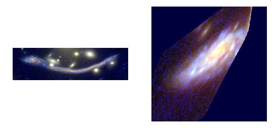
This is a gravitational arc called ‘the dragon’ lensed by the cluster Abell 370. On the left, you can see it in image plane, i.e. as it is in the sky, magnified it all its messy glory. On the right, we have use a lensing model to correct this magnification and get ‘the real galaxy’. This is called the source plane image.

The spatial distortion makes the analysis of these objects more difficult, especially when several images of the same object (called multiple images) are available. FRApy deals with this issue through forward-modelling: we start with a model in source plane (the ‘undistorted’ galaxy), lens it to image plane using a lensing model and compare it with the data.

What you’ll need

1. Deflection maps. These are 2D fits images produced from a lensing model that map how much deflection (in arcseconds along both directions RA DEC, 1 map each) a little photon landing in position RA,DEC in the sky has suffered due to the gravitational lensing effect. This is the core of FRApy’s modelling and allows one to generate lensed images that can be compared with the observations. One does this by calculating where each pixel in image plane originated from in the source plane. A number of Frontier Fields models provide these maps you can check them here here (example given for Abell 370). It is also possible to create these maps using LENSTOOL using the dpl command.

2. An analytical model that you hope describes your data, such as a gradient for metallicity or an arctangent model velocity fields. FRApy comes with a number of these models, that we used in our own publications, but we also show how you can create and fit your own model.

Install

>> pip install -i https://test.pypi.org/simple/ FRApy

The project is also available GitHub.

It requires the following packages:

• numpy==1.15.4
• matplotlib==3.0.2
• astropy==3.1
• reproject==0.4
• emcee==2.2.1
• pickle==4.0
• corner==2.0.1

Quick start

FRApy is a python module. A minimum working example would look something like this:

# Import FRApy
from frapy import Observation,Metallicity_Gradient,Output
from frapy import fit_model,make_input_parameters

# Load Observations
obs = Observation(z=0.611,
                  data_path='Demo_data/AS1063_map_metallicity.fits',
                  unc_path='Demo_data/AS1063_map_metallicity_unc.fits',
                  seeing = 1.03/0.2)

# Choose a Model, in this case a linear metallicity gradient
model = Metallicity_Gradient(zlens=0.322,
                             dfx_path='Demo_data/AS1063_dplx.fits',
                             dfy_path='Demo_data/AS1063_dply.fits')
model.create_projection_maps(obs)

# Fit the data
input_par = make_input_parameters(name    = ('cx', 'cy',  'q', 'pa', 'z_grad', 'z_0'),
                                  value   = (  29,   23,  0.7,   20,    -0.02, 9.0),
                                  minimum = (  28,   22,  0.4,  -20,     -0.1, 8.5),
                                  maximum = (  33,   27,  0.9,   90,      0.0, 9.5))
out = fit_model(obs,model,input_par,'output_file',nsteps=2000,nwalkers=24)

# Inspect the fit
results = Output('output_file')
results.best_parameters()

Mode in depth demos

We have included demo data used in Patricio et al. in prep. and two notebooks with examples on how to fit your data.

Metallicity Gradient Example.

Velocity Field Example.

Authors and Citations

This code was developed by:

• Vera Patricio (vera.patricio@dark-cosmology.dk)
• Johan Richard, lensing specialist

If you use FRApy in your science, please add the following citation:

Patrício et. al, 2018.

and

Patrício et. al, in prep.

and don’t forget astropy and emcee!

Observations

class frapy.observations.Observation(data_path, z, unc_path=None, seeing=0)

Data to be fitted.

This class handles the data that is going to be fitted with the models. It includes the image (data) to be fit, the associated uncertainty (optionally ), the redshift of the object and the seeing.

Parameters:

• data_path (str) – Path to the fits file containing the data.
• unc_path (str) – Path to the fits file containing the associated uncertainty (optional).
• z (float) – Redshift.
• seeing (float) – Seeing (in pixels). To be used in the model convolution.
• data (float array) – Data to be fitted. It is read from the data_path
• unc (float array) – Data uncertainted. It is read from the unc_path.

info()

Prints the data file, redshift and seeing.

plot(data_lim=None, unc_lim=None)

Plots the data and uncertainty. :param data_lim: minimum and maximum values of the data colour bar. :type data_lim: (float,float) :param unc_lim: minimum and maximum values of the uncertainty colour bar. :type unc_lim: (float,float)

Models

The BaseModel handles all the lensing part, producing a distance map that is used by all the other models.

class frapy.models.BaseModel(zlens, dfx_path, dfy_path, df_ang=0, cx=0, cy=0, q=1, pa=0)

Global lensing model to be used in all other Model classes .

This class prepares the deflection maps to be used with a particular object (i.e. at a particular redshift) and observations (i.e. aligns the maps with the data).

The main output is a distance map, in kiloparsecs, and an azimuthal map that serve as base for all the models being fit (metallicity gradient, velocity…)

Parameters:

• z_lens (float) – Redshift of the gravitational lens.
• dfx_path (str) – Path to the fits file with the x deflection.
• dfy_path (str) – Path to the fits file with the y deflection.
• cx (int) – x position of the centre (in pixels)
• cy (int) – y position of the centre (in pixels)
• q (float) – axis ratio (b/a)
• pa (float) – Position angle (0 North, +90 East )
• df_ang (float) – Angle between x axis and North (measured anti-clockwise) in the deflection maps.
• project_x (float array) – Lensing model (deflection in x direction) to be used to a particular object. Created with the ‘create_deflection_maps_for_object’ method.
• project_y (float array) – Lensing model (deflection in y direction) to be used to a particular object. Created with the ‘create_deflection_maps_for_object’ method.
• data (array) – An array with a realisation of a model made from the current parameter values.
• conv_data (array) – An array with a realisation of a model made from the current parameter values, convolved by the seeing of observations.

convolve_with_seeing(seeing)

Convolves a model with a Gaussian with width (sigma) ‘seeing’.

create_projection_maps(Observation, correct_z=True)

Takes the more global deflection maps produced by a graviatational lensing fitting code, and converts these maps to ‘projection’ maps, that maps where a pixel in source plane should be ‘projected’ in image plane, for this particular Observation. The project_x and project_y attributes are created with this function.

lensing_info()

Prints the lens redshift and deflection maps origin

make_azimuthal_map()

Produces an azimuthal map, in kpc, centrered in ‘cx’,’cy’ and assuming a ratio of ‘q’ between the minor and major axis, with the major axis in the ‘pa’ direction.

make_distance_map()

Produces a distance map, in kpc, centrered in ‘cx’,’cy’ and assuming a ratio of ‘q’ between the minor and major axis, with the major axis in the ‘pa’ direction.

plot()

Plots the model

class frapy.models.Metallicity_Gradient(zlens, dfx_path, dfy_path, df_ang=0, cx=0, cy=0, q=1, pa=0, z_grad=-1, z_0=0)

Linear metallicity gradient.

This model inherits the distance maps attributes (cx,cy,q and pa), from which the metallicity at each point is calculated assuming a gradient and a central metallicity value:

Z(r) = Delta Z * r + Z_0

with r the radius in kpc, Delta Z the gradient in dex/kpc, Z_0 the central metallicity.

Parameters:

• cx (int) – x position of the centre (in pixels)
• cy (int) – y position of the centre (in pixels)
• q (float) – axis ratio (a/b)
• pa (float) – Position angle (0 North, +90 East )
• z_grad (float) – Gradient in dex/kpc.
• z_0 (float) – Central metallicity value (value at cx,cy)

make_model()

Makes a model using the current parameters’ values and stores it in the ‘data’ attribute

model_name()

Returns the model’s name

model_parameters(verbose=True)

Returns the model’s parameters

print_parameter_values()

Returns the model’s parameters values

update_model_parameters(par)

Updates the parameters of the model.

Parameters:par (dictionary) – dictionary in the shape {‘name’:parameter_name, ‘value’:parameter value}

class frapy.models.Metallicity_Gradient_Constant_Centre(zlens, dfx_path, dfy_path, cx=0, cy=0, q=1, pa=0, z_grad=-1, z_0=0, r_flat=0.5, z_grad_inner=-1)

Linear metallicity gradient with a flatenning of the centre at r_flat.

This model inherits the distance maps attributes (cx,cy,q and pa), from which the metallicity at each point is calculated assuming a gradient and a central metallicity value:

Z(r) = Delta Z * r + Z_0

with r the radius in kpc, Delta Z the gradient in dex/kpc, Z_0 the central metallicity.

For r < r_flat, the metallicity is constant.

Parameters:

• cx (int) – x position of the centre (in pixels)
• cy (int) – y position of the centre (in pixels)
• q (float) – axis ratio (a/b)
• pa (float) – Position angle (0 North, +90 East )
• z_grad (float) – Gradient in dex/kpc.
• z_0 (float) – Central metallicity value (value at cx,cy)
• r_flat (float) – Radius that delimits the central zone where the metallicity is flat

make_model()

Makes a model using the current parameters’ values and stores it in the ‘data’ attribute

model_name()

Returns the model’s name

model_parameters(verbose=True)

Returns the model’s parameters

print_parameter_values()

Returns the model’s parameters values

update_model_parameters(par)

Updates the parameters of the model.

Parameters:par (dictionary) – dictionary in the shape {‘name’:parameter_name, ‘value’:parameter value}

class frapy.models.Velocity_Arctangent(zlens, dfx_path, dfy_path, cx=0, cy=0, q=1, pa=0, v_t=100, r_t=10)

Exponential velocity model.

This model inherits the distance and azimuthal maps, from which an arctangent model of the velocity at each point is calculated assuming the following formulae:

V(r) = v_t frac{2}{pi} arctan (frac{2r}{r_t})

with r the radius in kpc, v_t the terminal velocity and r_t the transition radius.

Parameters:

• cx (int) – x position of the centre (in pixels)
• cy (int) – y position of the centre (in pixels)
• q (float) – axis ratio (a/b)
• pa (float) – Position angle (0 North, +90 East )
• v_t (float) – Terminal velocity in km/s.
• r_t (float) – transition radius in kpc.

make_model()

Makes a model using the current parameters’ values and stores it in the ‘data’ attribute

model_name()

Returns the model’s name

model_parameters(verbose=True)

Returns the model’s parameters

print_parameter_values()

Returns the model’s parameters values

update_model_parameters(par)

Updates the parameters of the model.

Parameters:par (dictionary) – dictionary in the shape {‘name’:parameter_name, ‘value’:parameter value}

Fitting

frapy.fit_model.fit_model(obs, model, parameters, outputname, nsteps=1000, nwalkers=24, mask=None, binning_map=None)

Routine that fits the observations using a given model and the emcee sampler.

We make use of the emcee sampler (http://dfm.io/emcee/current/) to fit the free parameters of the model to the observations. We are maximising the following log-probabiluty function:

$ln(probability) = ln(priors) + ln(likelihood)$

with the log likelohood function as:

$ln(likelihood) = -frac{1}{2} ( frac{(data-model)^2}{uncertainty^2} + ln(2 pi uncertainty^2))$

Both the model and the observations should be instances of the Observations and BaseModel classes from frapy.

The parameters input is a dictionary in the shape:

parameters = {parameter_name1:{‘value’:X, ‘min’:Y, ‘max’:Z}, parameter_name2:{‘value’:A, ‘min’:B, ‘max’:C},…}

where the parameter_name variables should correspond to the parameters in the model being used; value is the starting value of each parameter; and min and max the minimum and maximum values allowed. We assume uniform priors to all parameters (i.e. all values between min and max have the same prior probability). Parameters not present in this dictionary will not be varied and will be kept to the value of the input model.

It is possible to mask part of the data out by using a mask. This should be a 2D array, of the same shape as the data, with only zeros (masked values) and ones (valid values). The maximisation will be made using only the valid values.

If the data was binned when deriving the quantity being fit, i.e. if pixels were grouped and analysed as a single pixel and that value taken as the value of all the pixels grouped, it is possible to include this information using a binning_map. This should be a 2D array in which pixels of the same bin are given the same value. Pixels in the image that were not analysed (not included in the binning) should be given negative values. These are not included in the minimisation.

Parameters:

• obs (Observation) – An instance of the Observation class
• model (Metallicity_Gradient,Velocity) – A frapy model (based in the BaseModel class)
• parameters (dictionary) – A dictionary containing the parameters of the model to be varied and their limits. Parameters not in this dictionary will not be varied.
• outputname (str) – Name of the output pickle file.
• nsteps (int) – number of steps of the emcee walkers. Default: 1000
• nwalkers (int) – Number of emcee walkers. Default: 24
• mask (array int) – Array of the same shape as the data containing only zeros (masked values) or ones (valid values). Optional.
• binning_map (array int) – Array of the same shape as the data containing encoding the pixels that were groupped togther. Optional.

Returns:

• Returns a dictionary with – sampler chain sampler lnprobability parameter names in the correct order input parameters the mask used the binning map used the observations the model
• This is also saved as a pickles file.

Explore the output

class frapy.check_fit.Output(outfile)

Allows the output of fit_model to be inspected

Reads the pickle output and allows to plot:

. the walkers positions at each iteration to check for convergence . a corner plot of the results . the 50th, 16th and 84th percentiles (mean and +/- 1 sigma)

Parameters:outfile (str) – The name of the pickle file being inspected (without the ‘.pickle’ extension)

best_parameters(start=0)

Calculates the 16th, 50th and 84th percentiles for each parameter. Only uses iterations after ‘start’

check_convergence()

Plots the walkers positions at each iteration for each parameter as well as the value of the log-likelihood probability for each iteration.

goodness_of_fit(best_parameters)

Given a dictionary with parameter names and values, calculates the chi2, reduced chi2 (chi2/dof), the log-likelihood probability and the Bayesian Information Criteria (BIC) for the model with those parameters values.

Parameters:best_parameters (dictionary) – Dictionary in the shape {parameter_name1:{value:X,min:Z,max:Z},parameter_name2:{value:X,min:Z,max:Z}} (from the check_fit.best_parameters function, for example). Returns:chi2/dof – Reduced chi2 Return type:float

make_cornerplot(start=0)

Makes a corner plot of the results. Only uses iterations after ‘start’

plot_solution(best_parameters)

Given a dictionary with parameter names and values, plots the model.

Parameters:best_parameters (dictionary) – Dictionary in the shape {parameter_name1:{value:X,min:Z,max:Z},parameter_name2:{value:X,min:Z,max:Z}} (from the check_fit.best_parameters function, for example). Returns:

• model (array float) – the model with the best parameters
• residuals (array float) – the residuals (data - model)

Miscelaneous

This module containts miscelaneous functions used in the fitting.

frapy.utils.make_input_parameters(name, value, minimum, maximum)

Outputs a parameter dictionary to be used in the fit_model function.

This dictionary has the following form:

{parameter_name1:{‘value’:X, ‘min’:Y, ‘max’:Z}, parameter_name2:{‘value’:A, ‘min’:B, ‘max’:C}, … }

Parameters:

• name (array str) – An array of strings containing the names of the model’s parameters to be fitted.
• value (array float) – The initial values of these parameters (ACTUALLY NOT USED)
• minimum (array float) – The minimum value allowed for each parameter
• maximum (array float) – The maximum value allowed for each parameter

Returns:

parameter

Return type:

dictionary

Indices and tables

• Index
• Module Index
• Search Page